Evaluation of Arbitrage Strategies on USDⓈ-M Market

Summary

• We evaluate basis and funding fee arbitrage strategies in Binance’s USDⓈ-M perpetual market with detailed simulations and results for BTC and ETH. The strategies discussed are 1) basis arbitrage, 2) simple holding funding fee arbitrage, and 3) a rebalancing approach to manage collateral.

• Effective arbitrage requires the portfolio margin or cross-asset margin mode, which considers the collective risk of multiple positions, allowing the use of crypto assets as collateral.

• Our back-testing analysis shows that the three strategies under our specified parameters can produce excellent risk-adjusted returns in both BTC and ETH. This demonstrates that these strategies can potentially be applied to other crypto assets.

Perpetual Markets

In the Binance exchange, there are primarily two types of perpetual futures markets: COIN-M and USDⓈ-M. In the COIN-M market, the funding fee and trading profit and loss (PNL or P&L) are settled using the crypto asset traded, whereas in the USDⓈ-M market, these are settled with stablecoins such as USDT and USDC. Following the previous article, Optimizing Funding Fee Arbitrage, where arbitrage strategies are evaluated in the COIN-M market, in this article, we evaluate basis and funding fee arbitrage strategies in the USDⓈ-M market.

Portfolio Margin Modes

To efficiently manage capital when executing arbitrage strategies in the USDⓈ-M market, it is essential to use portfolio margin mode or cross-asset margin mode. The primary difference from the traditional single asset mode, especially for risk-free arbitrage, is that the risk of multiple positions is considered collectively. This is particularly beneficial for trading strategies involving hedged positions, where the risk of the portfolio is reduced due to offsetting positions. Consequently, we can use crypto assets purchased from the spot market as collateral to support the short position in the USDT perpetual market. In contrast, the traditional single asset mode would require additional USDT as collateral for the short position.

Basis Arbitrage

The basis refers to the difference between the price of a futures contract and the spot price of the underlying asset, defined as:

$$B_t:=F_t-S_t$$

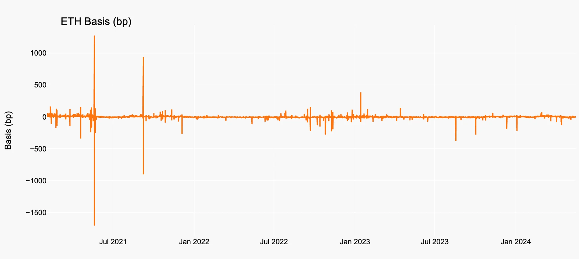
, where $B_t$ represents the basis, $F_t$ is the futures price, and $S_t$ is the spot price at time $t$. Figure 1 and Figure 2 show the historical basis for BTC and ETH.

Figure 1. BTC Basis History
Source: Binance, Presto Research

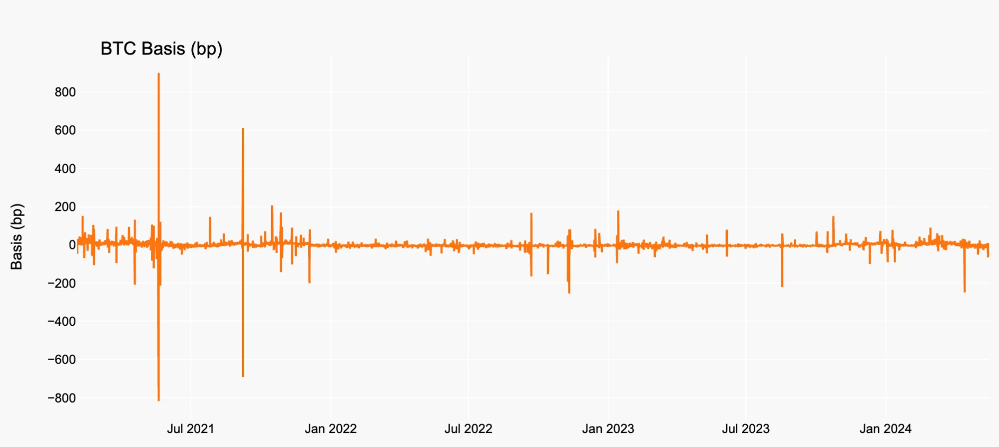
Figure 2. ETH Basis History
Source: Binance, Presto Research

We can set up a simple basis arbitrage strategy that longs the spot and shorts the perpetual when $B_t \ge \theta^u S_t$ and exit the position when $B_t \le \theta^l S_t$, where $\theta^u$ is the threshold for entering the position, whereas $\theta^l$ is the threshold for exiting. The P&L at time $t$ of this strategy can be broken down as follows:

$$PNL_t=PNL^{funding}_t+PNL^{basis}_t - TransactionCost_t \space\space\space\space\space (1)$$

, where $PNL^{funding}_t$ and $TransactionCost_t$ are self-explanatory, $PNL^{basis}_t$ comes from the change in the difference between the spot and perpetual prices.

The simulation results using $\theta^u:=0.005$ and $\theta^l:=-0.001$, and 1 million USDT book size on BTC and ETH are illustrated in Figure 3 and 4, and Table 1 and 2.

Figure 3. BTC Basis Arb
Source: Presto Research

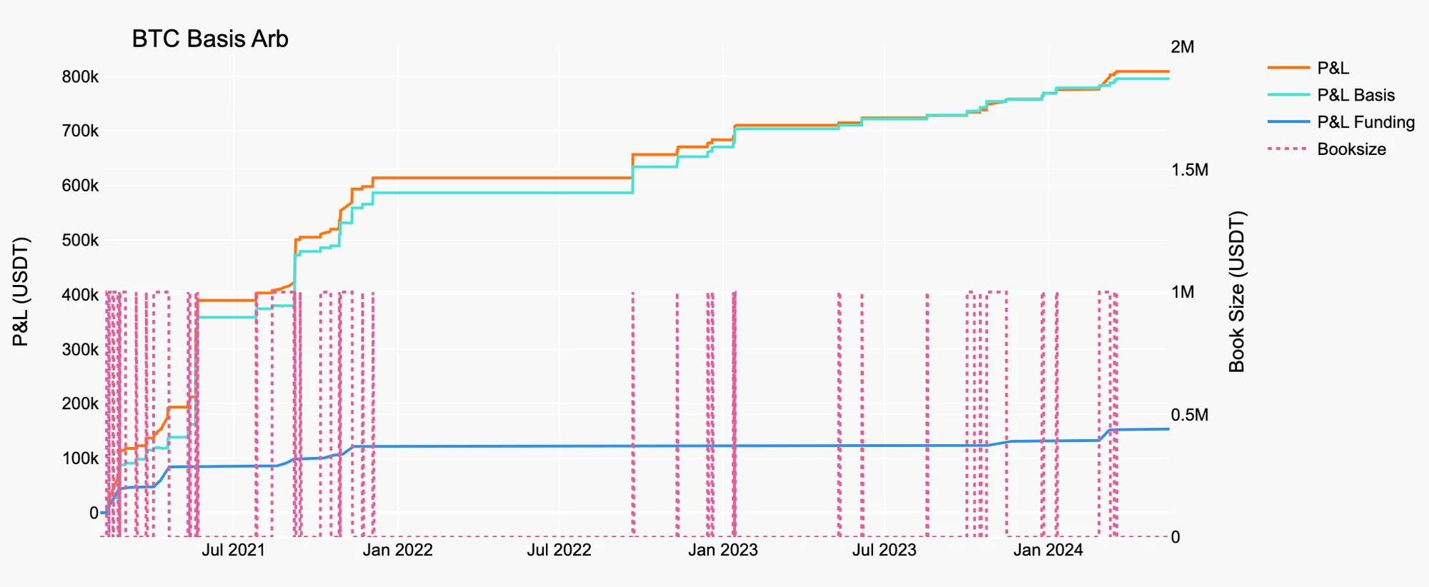
Table 1. Statistics of BTC Basis Arb

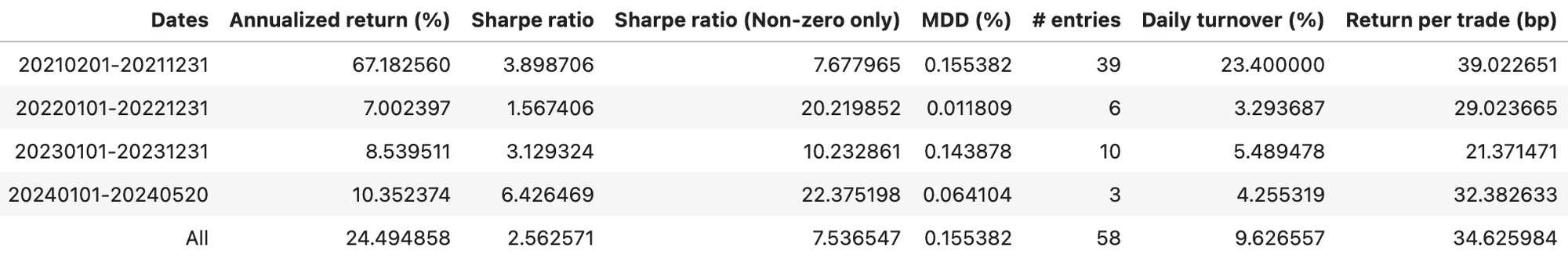
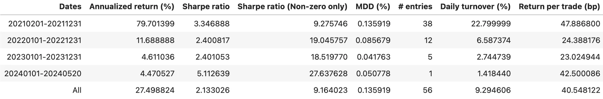
Figure 4. ETH Basis Arb
Source: Presto Research

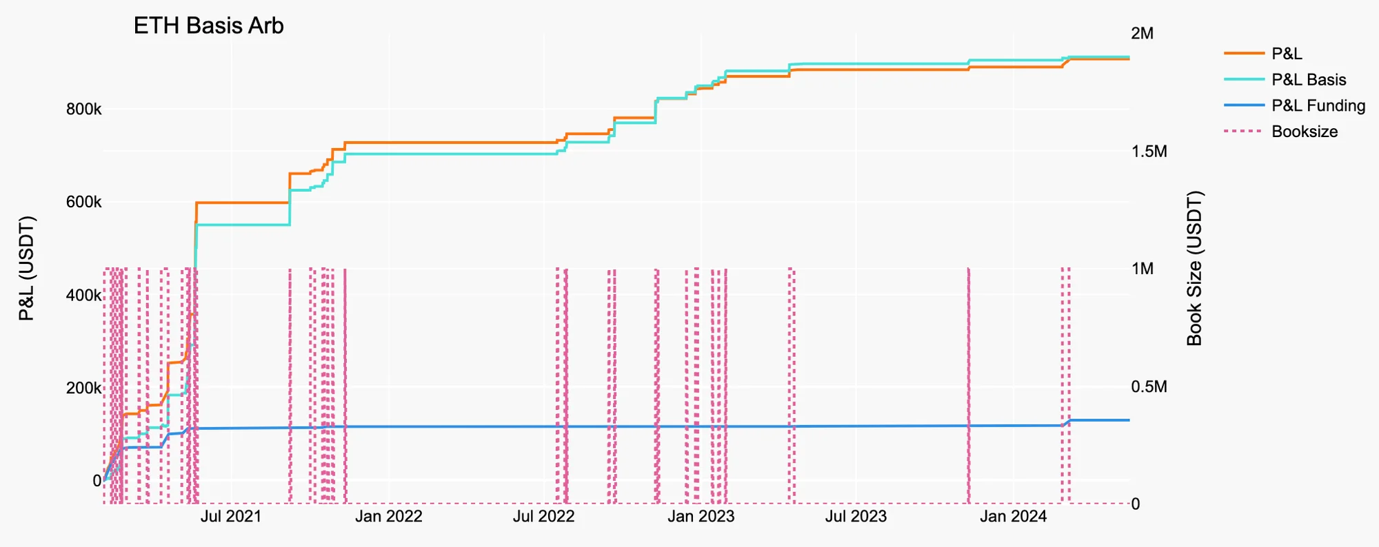
Table 2. Statistics of ETH Basis Arb

Funding Fee Arbitrage

The methodology for the funding fee arbitrage in the USDⓈ-M market is analogous to that used in the COIN-M market. A key difference is that the funding fee is settled with a stablecoin, thus eliminating the need to regularly sell the accrual. Therefore, the P&L of this strategy is the same as in equation (1) and it does not have the $PNL^{mark-to-market}_t$ component, unlike the strategies employed in the COIN-M market. For more details, refer to the previous article, Optimizing Funding Fee Arbitrage.

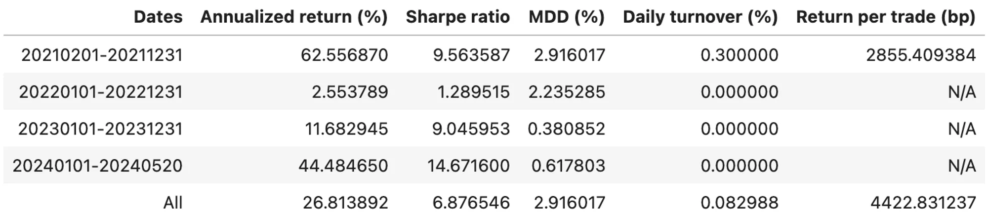
Strategy 1: Simple Holding

For optimal capital efficiency, this strategy requires the portfolio margin mode. Basically, this strategy mirrors the simple holding arbitrage strategy discussed in the previous article. To enter the arbitrage position, we purchase a crypto asset equivalent to 1 million USDT and use it as collateral to back the short position in the perpetual market. The results of this strategy applied to BTC and ETH are summarized in Figure 5 and 6, and Table 3 and 4.

In the figures, GMV (Gross Market Value) represents the absolute sum of Long Market Value (LMV) and Short Market Value (SMV):

$$\begin{aligned} GMV_t = LMV_t + |SMV_t|  \\ LMV_t = Q_t * S_t \\ SMV_t = -Q_t * F_t \end{aligned}$$

, where $Q_t$ is the quantity of the spot asset which is constant for this strategy. The book size used to calculate the return in the tables is assumed to be 1 million USDT, as unwinding the arbitrage position would give back almost the same amount, assuming no friction.

Figure 5. Simple Holding Funding Fee Arb on BTC
Source: Presto Research

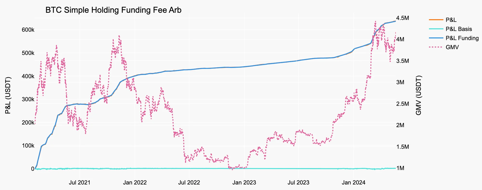
Table 3. Stats of Simple Holding Funding Fee Arb on BTC

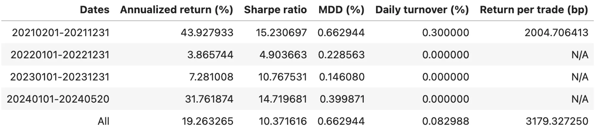
Figure 6. Simple Holding Funding Fee Arb on ETH
Source: Presto Research

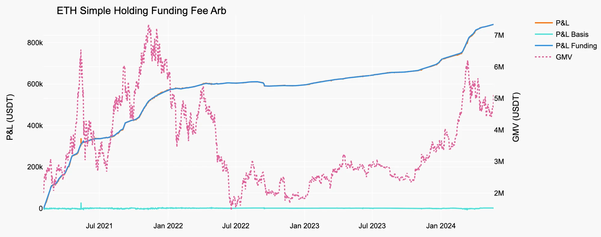
Table 4. Stats of Simple Holding Funding Fee Arb on ETH

Strategy 2: Rebalancing

If we cannot utilize the portfolio margin mode for some reasons such as operating on different exchanges, not meeting the required average transaction volume, etc., we must use a stablecoin as collateral for backing our short position. Proper management of this collateral is essential. To simplify the collateral management, rebalancing the GMV can be effective. By maintaining the same LMV and ensuring 30% of the SMV as the collateral, the book size would be calculated as:

$$BookSize_t:=LMV_0+0.3\cdot |SMV_t|$$

, where $LMV_0$ is the initial capital of 1 million USDT to purchase the asset in the spot market. The results of rebalancing the GMV of the portfolio daily are presented in Figure 7 and 8, and summarized in Table 5 and 6.

Figure 7. Rebalancing Funding Fee Arb on BTC
Source: Presto Research

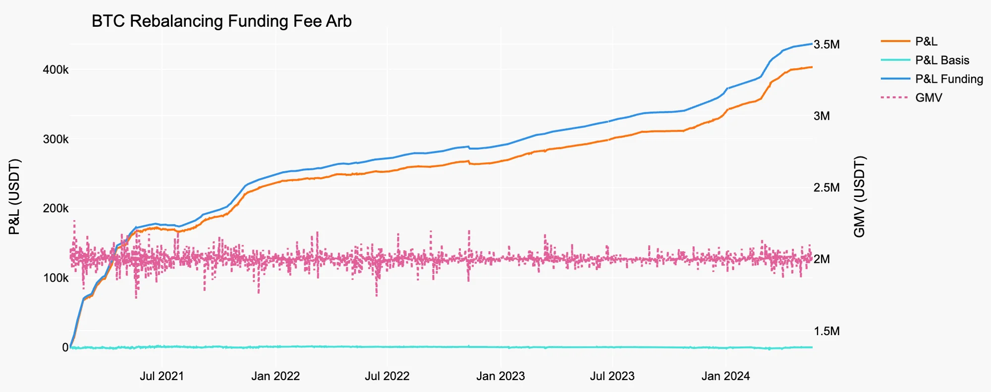
Table 5. Stats of Rebalancing Funding Fee Arb on BTC

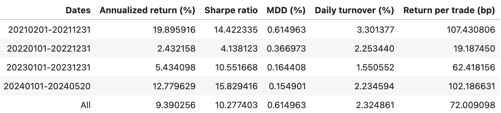
Figure 8. Rebalancing Funding Fee Arb on ETH
Source: Presto Research

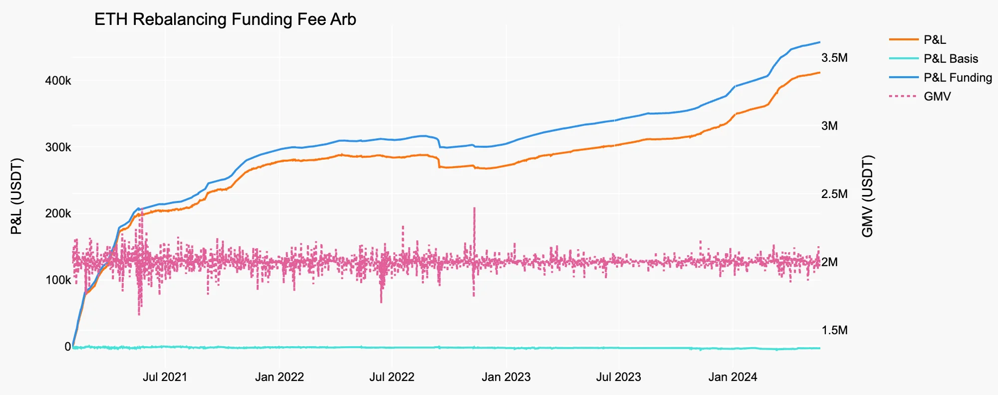
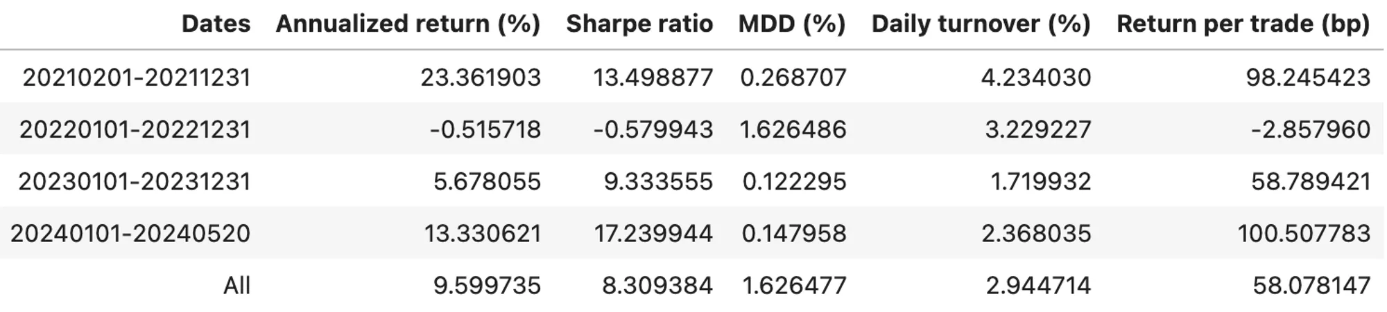
Table 6. Stats of Rebalancing Funding Fee Arb on ETH

Another reason to use the rebalancing approach is to increase the spot quantity when the spot price drops significantly, even if the portfolio margin mode is available. By increasing the quantity, we can potentially gain more profit from funding fees if the price rises. In such a case, frequent rebalancing would be unnecessary.

Conclusion

We have assessed the strategy that monetizes the basis changes and those that steadily earn from funding fees in the Binance USDⓈ-M market. In addition to BTC, we evaluated these strategies on ETH to demonstrate their expandability to other crypto assets. Our back-testing analysis shows that these strategies can produce excellent risk-adjusted returns. Improving the simple holding funding fee arbitrage by rebalancing the portfolio when the price drops below a certain percentage of the previous entry price is a topic for future research.